Transient methods for measuring thermal properties
Transient methods are widely used for measuring thermal properties of materials due to their efficiency and adaptability across various media. Among these, the line heat source method, commonly implemented via heated needle probes, is a well-established technique for determining thermal conductivity, thermal diffusivity, and volumetric specific heat. This article outlines the principles, instrumentation, and modeling approaches associated with this method.
Principle of the line heat source method
The line heat source method involves inserting a slender probe—typically referred to as a heated needle—into the material under study. The probe contains a heater running along its length and one or more temperature sensors. Configurations may include:
- A single needle with a central temperature sensor.
- Multiple temperature sensors placed at fixed intervals along the needle.
- A dual-needle setup, with one needle housing the heater and the other containing the temperature sensor.
Once the probe is embedded in the sample, a known quantity of heat is applied over a defined time period. The temperature response is recorded and compared to a theoretical model of a line heat source. The thermal properties of the model are iteratively adjusted until the simulated temperature response matches the measured data, thereby revealing the thermal properties of the material.
Data interpretation and modeling
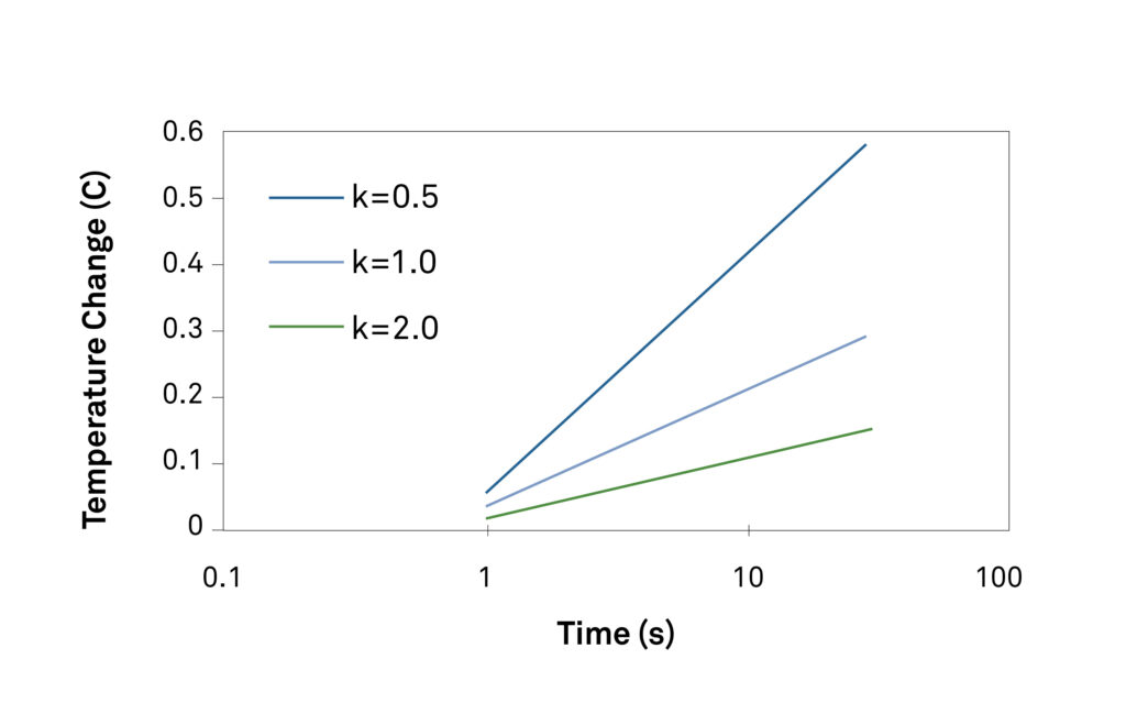

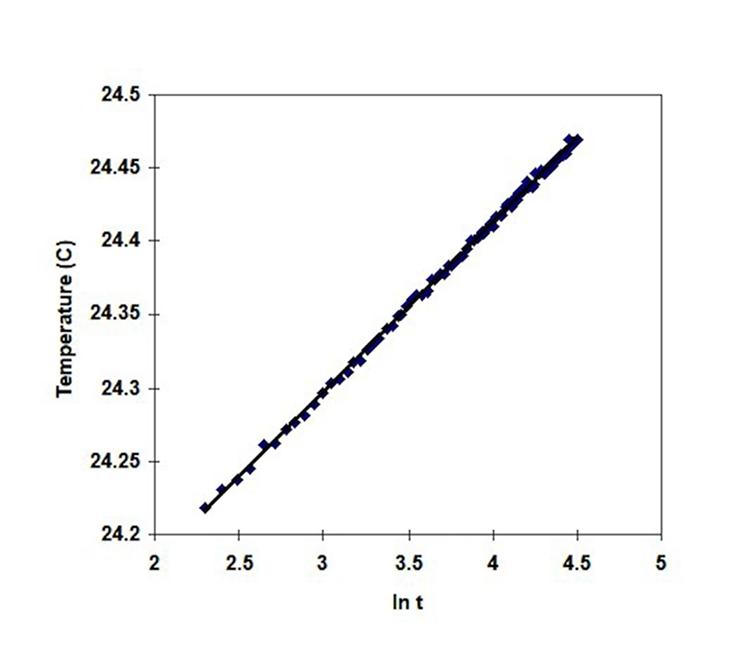
When using a single needle, such as the TEMPOS TR-3 large single needle (10 cm), the temperature change over time is plotted on a semi-logarithmic scale. The slope of the resulting line is inversely proportional to the material’s thermal conductivity. For example:
- A steeper slope indicates lower thermal conductivity
- Shallower slopes correspond to higher conductivity values
The theoretical model is based on the solution for an idealized line heat source:
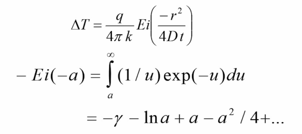
- q: Heat input per unit length
- k: Thermal conductivity
- r: Needle radius
- D: Thermal diffusivity
- t: Time
- Ei: Exponential integral (approximated by a series expansion)
- γ: Euler constant (0.5772)
For typical measurement durations, the first two terms of the exponential integral series provide a sufficient approximation.
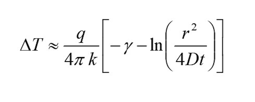
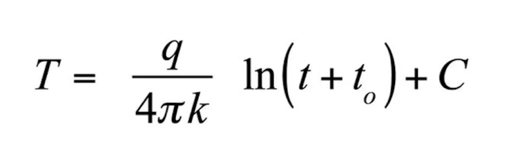
Rearranging the model yields a linear relationship between temperature and the logarithm of time.
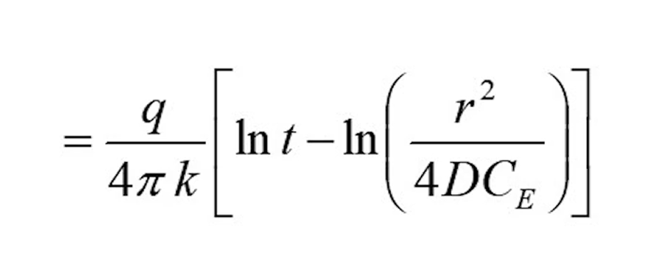
This allows conductivity to be calculated as:
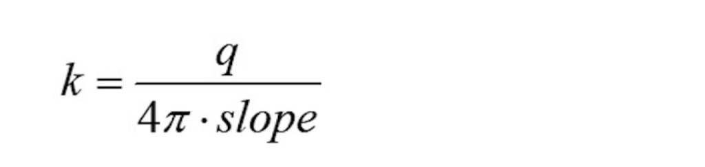
This model assumes a massless, infinitely small, and infinitely long heat source—an idealization that simplifies analysis but deviates from real probe behavior.
Enhancing model accuracy
To improve model fidelity, a time offset (to) can be introduced. This adjustment allows the use of early data points, which exhibit the most significant temperature changes. Without a time offset, analysts typically discard the initial third of the data to achieve a better fit. Incorporating the offset keeps the entire dataset intact, which reduces the time necessary for measurements and improves accuracy.
The trade-off is the need for a non-linear solver, as the modified equation becomes non-linear. However, this added complexity is justified by the enhanced performance.
Dual-needle configuration
An alternative approach involves two needles, such as the TEMPOS SH-3 dual-needle (3 cm), with one serving as the heater and the other as the temperature sensor.

In this approach:
- Temperature change is plotted on a linear time scale.
- The magnitude of the temperature peak is inversely proportional to the volumetric specific heat of the material.
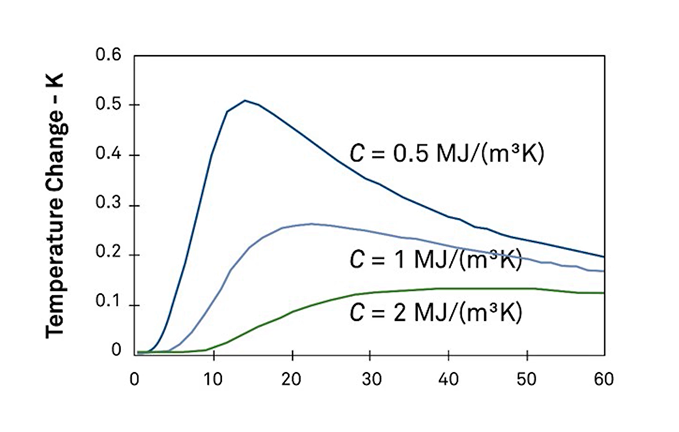
The model includes two equations—one for the heating phase and one for the cooling phase after the heat source is turned off. A computational optimization routine adjusts the thermal conductivity (k) and thermal diffusivity (D) until the predicted temperature curve aligns with the measured data.
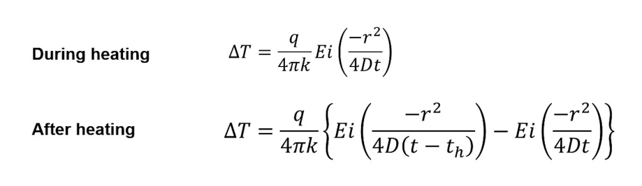
- q = heat input to needle (W/m)
- r = heater to temperature sensor distance
- th = heating time
- k = thermal conductivity
- D = thermal diffusivity
Both conductivity and diffusivity are used to calculate the material’s heat capacity.

